How EDI works to boost spectral resolution It reverses (during analysis) the heterodyning effect occuring in the instrument, to convert the broad moire patterns in the data back into the original high spatial frequency signals that formed them. |
||
Example of heterodyning, between two high spatial frequency patterns |
||
 |
|
|||||||
|
||||||||
Heterodyning forms beats, which are also called moire patterns |
||||||||

|
|||||
Lets follow what happens to an arbitrary signal in spatial-frequency space |
||
First, lets follow the signal through a conventional spectrograph. |
||
 |
||||
 |
Due to blurring from the spectrograph (from the slit width, or lens aberrations, or a poor quality grating), only the lowest spatial frequencies underneath the dashed Gaussian peak are detected by the conventional spectrograph. This is the problem: the narrow hatched areas are not detected. |
|||
 |
||||
Now lets follow the heterodyned signal through the EDI |
||
 |
||||||
The heterodyning that occurs between the sinusoidal interferometer transmission and the input signal effectively shifts the signal distribution toward lower spatial frequencies by a fixed amount, given by tau the interferometer delay. It also reduces its amplitude by half. |
||||||
The key point is that the blurring can be thought of as occuring AFTER the shifting is imposed. So structure in the hatched part of the distribution is preserved in the detected moire signal. |
||||||
 |
||
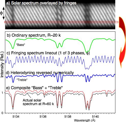
Example of reconstruction of higher resolution spectrum on the solar spectrum |
||
 |
||
Numerical simulation of 2.4x resolution boosting with photon noise |
||
Slide the animation frame counter to change the peak separation. This animation demonstrates that the equalization that was used to reshape the effective instrument lineshape into a Gaussian, and which creates a non-white noise distribution, does not prevent the EDI from behaving as a 2.4x boosted spectrograph. |
||
Site maintained by |
||||
Steps in numerically reversing the heterodyning
Before combining the ordinary and heterodyned signals together, we first mask them with individually different masks, to delete noise in regions where we expect there is no signal. A convenient mask is one that has a similar shape to the expected signal. One can use any mask shape, because the distribution is going to be equalized in the next step anyways, which effectively normalizes away any shape change you apply here.
(Remember that the ordinary signal also passes through the EDI, and we will use it later.)
The raw composite signal will be "lumpy", that is, non-Gaussian in effective lineshape. In particular, there is a valley of lower sensitivity at the foot of the ordinary response where it joins the foot of the heterodyned response. This valley is removed during the equalization step.
Similar to the graphic equalizer on a stereo sound system, we can increase or decrease the signal strength vs spatial frequency to force the effective instrument lineshape to be Gaussian. Behavior of the instrument on a calibrated spectrum provides information on how to choose the equalization curve.
Since both the signal and noise embedded with it are magnified/de-magnified the same amount, equalization is not cheating. The local S/N ratio for a specific spatial frequency is not altered by the equalization. However, a consequence is that the final noise distribution is no longer "white", as in the conventional spectrograph, but is non-uniform. The Figure after the next Figure, "Numerical Simulation of 2.4x ..." demonstrates that having a non-white noise distribution is not a problem. However, it is an interesting issue to explore.
The same noise pattern is applied to the "raw ccd data" in each case
Graphical example of heterodyning distinguishing a doublet
Details on extracting the fringing component:
We take 3 lineouts along the ccd dispersion direction, at 0, 120, and 240 degrees phase (or 4 lineouts at 0, 90, 180, 270 etc.), express each one as a complex wave, rotate each one by the opposite of the applied phase step so that they all align in the same phase, and add them. This separates the down-heterodyned signal from both the ordinary signal and the up-heterodyned conjugate.